Interpreting the Categorical Cross-Entropy Loss Function

A quick-hitter wherein I help figure out if your loss function sucks or not.

Loss functions usually mean something tangible. L2 loss is the mean square error of a fitting function, for example. But a number, by itself, usually doesn’t mean anything unless something sets the scale of what “large” means. Is an L2 loss value of 73.5 large or small? For L2, this is where the R-squared value comes in, at least for linear fitting, which basically asks “how good is our model compared to a model that just predicts the mean of the data?”. It’s a useful number, because it tells you how good your linear fit is compared to the simplest possible linear fit, which is a constant.

We can actually do something similar with the categorical cross-entropy, a favorite for classification problems. The categorical cross-entropy is the information entropy associated with putting each marble into a bucket and sorting them in the right buckets. If you don’t remember the formula, it’s

The categorical cross-entropy loss function, which I called S instead of L because I’m a physicist and it’s entropy.

$p^{(\sigma)}_i$ here is the softmax probability function prediction for data point $i$ to be in category $\sigma$, $x_i$ are the features, for sample $i$, and the $\hat{y}_i$ are the actual labels. If each label is totally 100% accurate with zero uncertainty, $\log(p^{(\sigma)}_i)$ is 0 and $(1 - \hat{y}_i)$ is zero, and the contribution to the entropy of that prediction is zero.

So perfect classification with infinite confidence would yield zero information entropy in the model. But that’s never going to happen, because data and models are not so accommodating. But we can ask a similar question to what the R-squared analysis asks, namely “What is the loss function for a trivial model?'“

In this case, let’s take our trivial multi-class classification model to return the $P_\sigma$ that comes from taking the probability of drawing that label randomly from the distribution of labels, viz. $P_i = N_\sigma/N$ for the $N_i$ members of category $\sigma$ and the whole sample size $N$.

The individual $P^{(\sigma)}$ are just constants, and by definition

$$\sum_i \hat{y}_i^{(\sigma)} = N P^{(\sigma)}$$

so we are left with the categorical cross-entropy of a random model trained on $N$ samples being

$$ {S}^* = - N \sum_\sigma P^{(\sigma)} \log P^{(\sigma)} + \left (1 - P^{(\sigma)} \right ) \log \left ( 1 - P^{(\sigma)} \right ) $$

This makes intuitive sense based on what we know entropy to be; a measure of the probability of any given marble occupying a specific slot, it’s just gratifying that we can get to it from the beginning. ${S}^*$ sorta fixes the scale for categorical cross-entropy classification loss functions. If the loss function is greater than ${S}^*$, the model is doing worse than our random model, and if it’s significantly lower than ${S}^*$, then it’s an improvement on a random sorter.

Finally, we can ask what this looks like for an equal distribution among all categories, so there is only one $P = 1/n$ for all $n$ categories. Well, it’s this decaying thing:

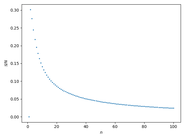
per-data-point categorical cross-entropy for even distribution across $n$ categories.

The entropy is 0 if there’s one category, which makes sense because the whole thing is perfectly ordered. Then it shoots upward and slowly decays towards 0 again as $n \rightarrow \infty$, which also makes intuitive sense if you spend time thinking about what the entropy tells you about sorting marbles into buckets. Depending on the number of categories you’re classifying, the per-data-point categorical cross-entropy will probably fall somewhere between about 0.3 and 0.1, unless you have a lot more categories.

Edit: To implement this for your own models, I put up a gist on GitHub for a custom Keras Metric that computes the normalized categorical cross-entropy, ${S}/{S^*}$, so you can monitor it while training.